Palettes in R

In its simplest form, a palette in R is simply a vector of colors. This vector can be include the hex triplet or R color names.

The default palette can be seen through palette():

> palette("default") # you'll only need this line if you've previously changed the palette from the default

> palette()
[1] "black"   "red"     "green3"  "blue"    "cyan"    "magenta" "yellow"
[8] "gray"

Defining your own palettes

If you want to make your own palette, you can just create your own vector of colors. It's fine for your vector to include a mixture of hex triplets and R color names. You can use the palette function above, but generally it's best to just store each palette as a standard vector. For one thing, you can use more than one palette that way. Here's how you can define your own palette:

colors <- c("#A7A7A7",
 "dodgerblue",
 "firebrick",
 "forestgreen",
 "gold")

Now let's try using our palette. For now let's just color each bar of a histogram. This is a silly example, but I think it's the easiest way to show how to get R to utilize your palette. In the following example, there are six bars, but only five colors. You can see that R will cycle through your palette to fill all the shapes.

hist(discoveries,
 col = colors)

A more sensible use of color is to use a different color for each of a number of summary statistics:

colors <- c("#A7A7A7",
 "dodgerblue",
 "firebrick",
 "forestgreen",
 "gold")
hist(discoveries,
 col = colors[1])
abline(v = mean(discoveries),
 col = colors[2],
 lwd = 5)
abline(v = median(discoveries),
 col = colors[3],
 lwd = 5)
abline(v = min(discoveries),
 col = colors[4],
 lwd = 5)
abline(v = max(discoveries),
 col = colors[5],
 lwd = 5)

legend(x = "topright", # location of legend within plot area
 col = colors[2:5],
c("Mean", "Median", "Minimum", "Maximum"),
 lwd = 5)

Predefined palettes: default R palettes

The package grDevices (you probably already have this loaded) contains a number of palettes.

?rainbow
rainbowcols <- rainbow(6)
hist(discoveries,
 col = rainbowcols)

For rainbow, you can adjust the saturation and value. For example:

rainbowcols <- rainbow(6,
 s = 0.5)
hist(discoveries,
 col = rainbowcols)

heatcols <- heat.colors(6)
hist(discoveries,
 col = heatcols)

As well as rainbow and heat.colors, there are also terrain.colors, topo.colors, and cm.colors.

Predefined palettes: RColorBrewer

library(RColorBrewer)
display.brewer.all()

The above lines will show us all the RColorBrewer palettes (output shown below). The top section of palettes are sequential, the middle section are qualitative, and the lower section are diverging. Here is some information about how to choose a good palette.

RColorBrewer palettes

RColorBrewer works a little different than how we've defined palettes previously. We'll have to use brewer.pal to create a palette.

library(RColorBrewer)
darkcols <- brewer.pal(8, "Dark2")
hist(discoveries,
 col = darkcols)

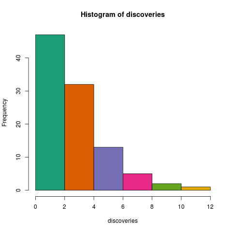
Even though we have to provide brewer.pal with the number of colors we want, we won't necessarily need to use all those colors later. We can still choose a color from the vector like we have previously. When we're setting a col setting to the full palette, we'll be more concerned with how many colors are included in the palette , but even there, we can choose a subset of the whole palette:

darkcols <- brewer.pal(8, "Dark2")
hist(discoveries,
 col = darkcols[1:2])

Here's the code from this post.

Now that we're familiar with making our own palettes and using the built-in palettes in grDevices and RColorBrewer, I'm planning a future post about a more practical (but also more complicated) example of using palettes: making maps.

--
This post is one part of my series on palettes.

Random Name Generator in R

Just for the heck of it, let's recreate my Reality TV Show Name Generator in R. This isn't really the sort of thing you'd normally do in R, but we can try out a bunch of different functions this way: random integers/sampling, concatenation, sorting, and determining the length of an object.

First, let's create a dictionary for R to randomly pull names from. In this case, we want a first word and a last word, that we'll later combine to create a name similar to so many current TV shows. (Note: In some cases, I've made the first "word" or last "word" multiple words for some variety.) Feel free to make your own lists.

first <- c("Fear", "Frontier", "Nanny", "Job", "Yard", "Airport", "Half Pint", "Commando", "Fast Food", "Basketball", "Bachelorette", "Diva", "Baggage", "College", "Octane", "Clean", "Sister", "Army", "Drama", "Backyard", "Pirate", "Shark", "Project", "Model", "Survival", "Justice", "Mom", "New York", "Jersey", "Ax", "Warrior", "Ancient", "Pawn", "Throttle", "The Great American", "Knight", "American", "Outback", "Celebrity", "Air", "Restaurant", "Bachelor", "Family", "Royal", "Surf", "Ulitmate", "Date", "Operation", "Fish Tank", "Logging", "Hollywood", "Amateur", "Craft", "Mystery", "Intervention", "Dog", "Human", "Rock", "Ice Road", "Shipping", "Modern", "Crocodile", "Farm", "Amish", "Single", "Tool", "Boot Camp", "Pioneer", "Kid", "Action", "Bounty", "Paradise", "Mega", "Love", "Style", "Teen", "Pop", "Wedding", "An American", "Treasure", "Myth", "Empire", "Motorway", "Room", "Casino", "Comedy", "Undercover", "Millionaire", "Chopper", "Space", "Cajun", "Hot Rod", "The", "Colonial", "Dance", "Flying", "Sorority", "Mountain", "Auction", "Extreme", "Whale", "Storage", "Cake", "Turf", "UFO", "The Real", "Wild", "Duck", "Queer", "Voice", "Fame", "Music", "Rock Star", "BBQ", "Spouse", "Wife", "Road", "Star", "Renovation", "Comic", "Chef", "Band", "House", "Sweet")

second <- c("Hunters", "Hoarders", "Contest", "Party", "Stars", "Truckers", "Camp", "Dance Crew", "Casting Call", "Inventor", "Search", "Pitmasters", "Blitz", "Marvels", "Wedding", "Crew", "Men", "Project", "Intervention", "Celebrities", "Treasure", "Master", "Days", "Wishes", "Sweets", "Haul", "Hour", "Mania", "Warrior", "Wrangler", "Restoration", "Factor", "Hot Rod", "of Love", "Inventors", "Kitchen", "Casino", "Queens", "Academy", "Superhero", "Battles", "Behavior", "Rules", "Justice", "Date", "Discoveries", "Club", "Brother", "Showdown", "Disasters", "Attack", "Contender", "People", "Raiders", "Story", "Patrol", "House", "Gypsies", "Challenge", "School", "Aliens", "Towers", "Brawlers", "Garage", "Whisperer", "Supermodel", "Boss", "Secrets", "Apprentice", "Icon", "House Party", "Pickers", "Crashers", "Nation", "Files", "Office", "Wars", "Rescue", "VIP", "Fighter", "Job", "Experiment", "Girls", "Quest", "Eats", "Moms", "Idol", "Consignment", "Life", "Dynasty", "Diners", "Chef", "Makeover", "Ninja", "Show", "Ladies", "Dancing", "Greenlight", "Mates", "Wives", "Jail", "Model", "Ship", "Family", "Videos", "Repo", "Rivals", "Room", "Dad", "Star", "Exes", "Island", "Next Door", "Missions", "Kings", "Loser", "Shore", "Assistant", "Comedians", "Rooms", "Boys")

Whew, that was long. Instead, let's look at a random sample of those.

We can make random lists using sample. Sample wants you to provide it with a vector, the sample size you want, and whether or not it should reuse items from the vector. In this case, we don't want any duplicates, so we add replace = FALSE.

first <- sample(first,
 10,
 replace = FALSE)

second <- sample(second,
 12,
 replace = FALSE)

This gives us something more like

> first
 [1] "Teen"       "Fame"       "Basketball" "Sister"     "Bachelor" 
 [6] "Half Pint"  "Myth"       "Paradise"   "Frontier"   "Fast Food"
> second
 [1] "Comedians"    "Boss"         "Experiment"   "Wives"        "Wedding"    
 [6] "Intervention" "Days"         "Raiders"      "Attack"       "Sweets"     
[11] "Jail"         "Whisperer"

It's random, so your list will probably be different.

If you want to sort them alphabetically, use

first <- sort(first)

If we had wanted to randomly resort the whole "first" list, we could have entered the command

first <- sample(first, length(first), replace = FALSE)

Using length makes it easy to resort the whole list. You don't have to look up how many items there are in first.

Let's use length again to choose a random number that we'll use to grab a number from the first list, and then again to choose a random number that we'll use to grab a number from the second list:

rand1 <- sample(1:length(first), 1)
rand2 <- sample(1:length(second), 1)

And finally, we want to pull an item from each list and concatenate them. We could concatenate to a file, but here we'll just let it print to the console.

cat(first[rand1], second[rand2], "\n")

"\n" produces a line break so we can do source(reality.R) again and have another name pop up on the next line.

If you've made a dictionary of your own and want to check for duplicates, you can do the following:

anyDuplicated(first) # if not 0, there are that many duplicates
duplicated(first) # this will show which items are duplicates

Feel free to improve on my dictionary or generator. I'd love to see it.

Code available as a gist.

Adding Measures of Central Tendency to Histograms in R

Building on the basic histogram with a density plot, we can add measures of central tendency (in this case, mean and median) and a legend.

Like last time, we'll use the beaver data from the datasets package.

hist(beaver1$temp, # histogram
 col = "peachpuff", # column color
 border = "black", 
 prob = TRUE, # show densities instead of frequencies
 xlim = c(36,38.5),
 ylim = c(0,3),
 xlab = "Temperature",
 main = "Beaver #1")
lines(density(beaver1$temp), # density plot
 lwd = 2, # thickness of line
 col = "chocolate3")

Next we'll add a line for the mean:

abline(v = mean(beaver1$temp),
 col = "royalblue",
 lwd = 2)

And a line for the median:

abline(v = median(beaver1$temp),
 col = "red",
 lwd = 2)

And then we can also add a legend, so it will be easy to tell which line is which.

legend(x = "topright", # location of legend within plot area
 c("Density plot", "Mean", "Median"),
 col = c("chocolate3", "royalblue", "red"),
 lwd = c(2, 2, 2))

All of this together gives us the following graphic:

In this example, the mean and median are very close, as we can see by using median() and mode().

> mean(beaver1$temp)
[1] 36.86219

> median(beaver1$temp)
[1] 36.87

We can do like we did in the previous post and graph beaver1 and beaver2 together by adding a layout line and changing the limits of x and y. The full code for this is available in a gist.

Here's the output from that code: