Sorting Within Lattice Graphics in R

Default

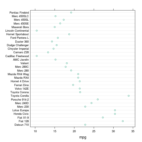
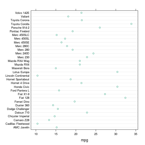
By default, lattice sorts the observations by the axis values, starting at the bottom left.

For example,

library(lattice)

colors = c("#1B9E77", "#D95F02", "#7570B3")

dotplot(rownames(mtcars) ~ mpg,
 data = mtcars,
 col = colors[1],
 pch = 1)

produces:

Default lattice dotplot

(Note: The rownames(cars) bit is just because of how this data set is stored. For your data, you might just type the variable name (model, for example) instead.)

Graphing one variable, sorting by another

If we want to show the same data, but we want to sort by another variable (or the same variable, for that matter), we can just add reorder(yvar, sortvar). For example, to sort by the number of cylinders, we could:

dotplot(reorder(rownames(mtcars), cyl) ~ mpg,
 data = mtcars,
 col = colors[1],
 pch = 1)

Sorted by number of cylinders

Graphing two variables

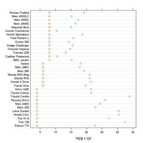
To better show how this works, let's graph cyl alongside mpg, so we can see how it is sorting:

dotplot(reorder(rownames(mtcars), cyl) ~ mpg + cyl,
 data = mtcars,
 col = colors,
 pch = c(1, 0))

Graph of mpg and cyl, sorted by cyl

Reverse order

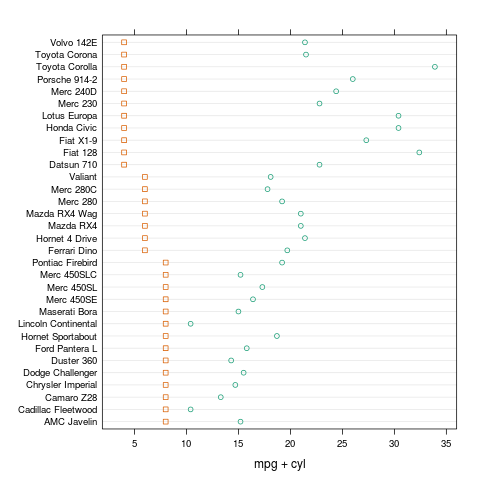
We can also sort in reverse order, by adding a "-" before the variable name:

dotplot(reorder(rownames(mtcars), -cyl) ~ mpg + cyl,
 data = mtcars,
 col = colors,
 pch = c(1, 0))

Graph of mpg and cyl, sorted by cyl, reversed

Adding a legend

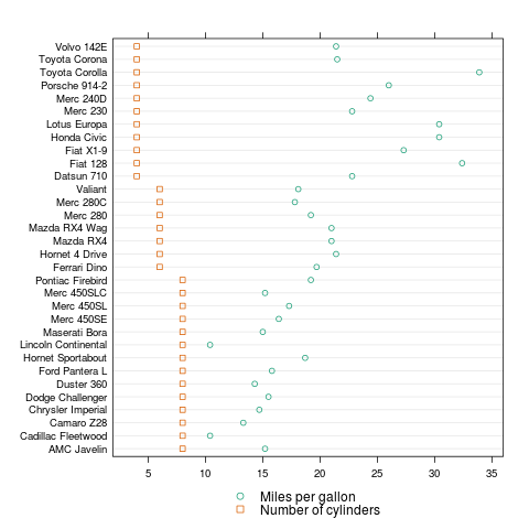
We can also add a legend:

dotplot(reorder(rownames(mtcars), -cyl) ~ mpg + cyl,
 data = mtcars,
 xlab = "",
 col = colors,
 pch = c(1, 0),
 key = list(points = list(col = colors[1:2], pch = c(1, 0)),
  text = list(c("Miles per gallon", "Number of cylinders")),
  space = "bottom"))

With legend

Other lattice types

The same technique will work with other lattice graphs, such as barchart, bwplot, and stripplot.

Full code available as a gist.

Subfigures in LaTeX

How can you create subfigures or subfloats in LaTeX? It's often easy to combine multiple figures from within a statistical package or image software, but it's generally best not to if you want to include subcaptions as text, for improved searchability.

Fortunately the subcaption package in LaTeX allows us to do this easily. (The subfigure and subfig packages have been deprecated, so it's best to use subcaption instead.)

How can you make more than one image or table be part of a LaTeX figure while still being able to create text captions for each?

Using the word clouds from my R word cloud tutorial, let's look at an example:

In order to make the figure containing the subfigures, we'll need to decide a few things first. Then it's just a matter of letting LaTeX know our preferences:

• The precise or proportional width of the subfigures
• The filenames
• The subcaptions
• How much horizontal or vertical space should be between subfigures
• The overall figure caption

We also need to let LaTeX know to use the caption and subcaption packages. The full code for the example image above is included below, and also in a gist.

\documentclass{article}

\usepackage{graphicx}
\usepackage{caption}
\usepackage{subcaption}

\begin{document}

\begin{figure}
 \centering
 \begin{subfigure}{0.4\textwidth} % width of left subfigure
  \includegraphics[width=\textwidth]{rncalt.png}
  \caption{RNC} % subcaption
 \end{subfigure}
 \vspace{1em} % here you can insert horizontal or vertical space
 \begin{subfigure}{0.4\textwidth} % width of right subfigure
  \includegraphics[width=\textwidth]{dncalt.png}
  \caption{DNC} % subcaption
 \end{subfigure}
 \caption{Wordcloud of national conventions} % caption for whole figure
\end{figure}

\end{document}

For more information, this wikibooks article is useful.


--
This post is one part of my series on LaTeX.

White Space in LaTeX

Extra spaces and line breaks in your source file are ignored. But there are several ways to force LaTeX to introduce white space to your documents.

The most simple commands to insert a specific amount of white space into your document are \hspace and \vspace.

To produce vertical space, use \vspace followed by the length of the space in brackets. This length can be represented in any units recognized by LaTeX, e.g. \vspace{2 in}. The space between the number and the unit is optional, so \vspace{2in} will also work.

Similarly, you can use \hspace to insert horizontal space in your document, e.g., \hspace{2 in}.

If \hspace and \vspace are not working as you would like (often at the beginning or end of a line or page), you can instead use \hspace* and \vspace*, which will force space to appear.

If you want to put in as much blank space as possible (while still maintaining page margins, etc.), you can use \hfill and \vfill.

Multiples of \vfill or \hfill on a particular page or in an environment will fill an even amount of the space. (E.g., if there are 6 inches to be filled and 3 \vfill's, each will take 2 inches.)

Horizontal

As well as \hspace{} and \hfill, there are some horizontal-specific commands for adding white space.

\quad creates a space whose size is relative to the current font size and font face. \quad is equal to \hspace{1em}. There are other commands that make spaces of sizes relative to \quad:

Horizontal space commands in LaTeX

Vertical

Probably the most common white space command is \\. It is used to start a new paragraph.

That's not the only way to tell LaTeX to break a line. Here are a number of ways to do that in different situations:

command	action
\\	Start a new paragraph
\linebreak[number]	Start a new line, option to request, not require
\newline	Line break (only in paragraph mode)

Line breaks in LaTeX

\newline or \linebreak can be beneficial because they work inside the tabular environment (when a p column definition is used), where \\ will not work within a cell.

As well as using \vspace{} and \vfill, there are some specific commands for vertical white space:

• \smallskip
• \medskip
• \bigskip

The sizes of \smallskip, \medskip, and \bigskip are determined by the documentclass.

Example of skip sizes

There are also several kinds of ways to break a page, which sometimes creates white space:

command	action
\pagebreak	Starts a new page, using white space throughout to fill the full page before the break
\newpage	Starts a new page, leaving the rest of the page before the break blank
\clearpage	Like \newpage, but also prints all prior figures
\cleardoublepage	Like \clearpage, but next page with print will be odd

Page breaks in LaTeX

Here's an example of the difference between \pagebreak and \newpage.

More information

• http://crab.rutgers.edu/~karel/latex/class5/class5.html
• http://help-csli.stanford.edu/tex/latex-pagebreaks.shtml
• http://www.personal.ceu.hu/tex/breaking.htm
• http://www.mollietaylor.com/2012/11/units-in-latex.html

--
This post is one part of my series on LaTeX.

Units in LaTeX

Discrete units

These are your basic units, like inches, centimeters, and points. Conversion of units from here and here.

These tables show the relative sizes of each unit:

Relative sizes of units in LaTeX, inches

Relative sizes of units in LaTeX, cm

Units defined relative to font sizes

There also are sizes that are relative to the current font face and font size. The size ex is usually the same as the height of an "x", and the size em is usually (but less often) equal to the width of an "M".

Since these are relative to your font, don't be surprised if your attempts look different than mine. Just like their absolute sizes, the size of ex relative to em is not consistent across fonts.

Examples of font-relative units

Units defined relative to document

There also are units that have definitions relative to your document. These are determined based on your documentclass, and can also be explicitly changed.

A list of these and how to change them is available here. Some of the sizes are illustrated here.

command	size
\paperwidth	Width of page
\paperheight	Height of page
\textwidth	Width of text
\textheight	Height of text
\linewidth	Width of a line, usually equal to \textwidth, but varies with environment
\columnwidth	Width of a column, usually same as \linewidth
\columnsep	Distance between columns
\tabcolsep	Separation between columns in a tabular environment
\parindent	Paragraph indentation
\parskip	The extra vertical space between paragraphs
\baselineskip	Vertical distance between lines in a paragraph
\baselinestretch	Multiplies \baselineskip
\unitlength	Units of length in a picture environment
\topmargin	Size of top margin
\evensidemargin	Margin of even pages
\oddsidemargin	Margin of odd pages

Document size commands in LaTeX

Next, we'll learn how to use these units to add white space.


--
This post is one part of my series on LaTeX.

Palettes in R

In its simplest form, a palette in R is simply a vector of colors. This vector can be include the hex triplet or R color names.

The default palette can be seen through palette():

> palette("default") # you'll only need this line if you've previously changed the palette from the default

> palette()
[1] "black"   "red"     "green3"  "blue"    "cyan"    "magenta" "yellow"
[8] "gray"

Defining your own palettes

If you want to make your own palette, you can just create your own vector of colors. It's fine for your vector to include a mixture of hex triplets and R color names. You can use the palette function above, but generally it's best to just store each palette as a standard vector. For one thing, you can use more than one palette that way. Here's how you can define your own palette:

colors <- c("#A7A7A7",
 "dodgerblue",
 "firebrick",
 "forestgreen",
 "gold")

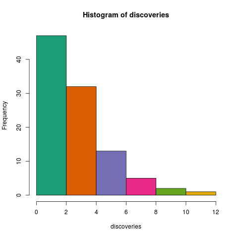
Now let's try using our palette. For now let's just color each bar of a histogram. This is a silly example, but I think it's the easiest way to show how to get R to utilize your palette. In the following example, there are six bars, but only five colors. You can see that R will cycle through your palette to fill all the shapes.

hist(discoveries,
 col = colors)

A more sensible use of color is to use a different color for each of a number of summary statistics:

colors <- c("#A7A7A7",
 "dodgerblue",
 "firebrick",
 "forestgreen",
 "gold")
hist(discoveries,
 col = colors[1])
abline(v = mean(discoveries),
 col = colors[2],
 lwd = 5)
abline(v = median(discoveries),
 col = colors[3],
 lwd = 5)
abline(v = min(discoveries),
 col = colors[4],
 lwd = 5)
abline(v = max(discoveries),
 col = colors[5],
 lwd = 5)

legend(x = "topright", # location of legend within plot area
 col = colors[2:5],
c("Mean", "Median", "Minimum", "Maximum"),
 lwd = 5)

Predefined palettes: default R palettes

The package grDevices (you probably already have this loaded) contains a number of palettes.

?rainbow
rainbowcols <- rainbow(6)
hist(discoveries,
 col = rainbowcols)

For rainbow, you can adjust the saturation and value. For example:

rainbowcols <- rainbow(6,
 s = 0.5)
hist(discoveries,
 col = rainbowcols)

heatcols <- heat.colors(6)
hist(discoveries,
 col = heatcols)

As well as rainbow and heat.colors, there are also terrain.colors, topo.colors, and cm.colors.

Predefined palettes: RColorBrewer

library(RColorBrewer)
display.brewer.all()

The above lines will show us all the RColorBrewer palettes (output shown below). The top section of palettes are sequential, the middle section are qualitative, and the lower section are diverging. Here is some information about how to choose a good palette.

RColorBrewer palettes

RColorBrewer works a little different than how we've defined palettes previously. We'll have to use brewer.pal to create a palette.

library(RColorBrewer)
darkcols <- brewer.pal(8, "Dark2")
hist(discoveries,
 col = darkcols)

Even though we have to provide brewer.pal with the number of colors we want, we won't necessarily need to use all those colors later. We can still choose a color from the vector like we have previously. When we're setting a col setting to the full palette, we'll be more concerned with how many colors are included in the palette , but even there, we can choose a subset of the whole palette:

darkcols <- brewer.pal(8, "Dark2")
hist(discoveries,
 col = darkcols[1:2])

Here's the code from this post.

Now that we're familiar with making our own palettes and using the built-in palettes in grDevices and RColorBrewer, I'm planning a future post about a more practical (but also more complicated) example of using palettes: making maps.

--
This post is one part of my series on palettes.

Random Name Generator in R

Just for the heck of it, let's recreate my Reality TV Show Name Generator in R. This isn't really the sort of thing you'd normally do in R, but we can try out a bunch of different functions this way: random integers/sampling, concatenation, sorting, and determining the length of an object.

First, let's create a dictionary for R to randomly pull names from. In this case, we want a first word and a last word, that we'll later combine to create a name similar to so many current TV shows. (Note: In some cases, I've made the first "word" or last "word" multiple words for some variety.) Feel free to make your own lists.

first <- c("Fear", "Frontier", "Nanny", "Job", "Yard", "Airport", "Half Pint", "Commando", "Fast Food", "Basketball", "Bachelorette", "Diva", "Baggage", "College", "Octane", "Clean", "Sister", "Army", "Drama", "Backyard", "Pirate", "Shark", "Project", "Model", "Survival", "Justice", "Mom", "New York", "Jersey", "Ax", "Warrior", "Ancient", "Pawn", "Throttle", "The Great American", "Knight", "American", "Outback", "Celebrity", "Air", "Restaurant", "Bachelor", "Family", "Royal", "Surf", "Ulitmate", "Date", "Operation", "Fish Tank", "Logging", "Hollywood", "Amateur", "Craft", "Mystery", "Intervention", "Dog", "Human", "Rock", "Ice Road", "Shipping", "Modern", "Crocodile", "Farm", "Amish", "Single", "Tool", "Boot Camp", "Pioneer", "Kid", "Action", "Bounty", "Paradise", "Mega", "Love", "Style", "Teen", "Pop", "Wedding", "An American", "Treasure", "Myth", "Empire", "Motorway", "Room", "Casino", "Comedy", "Undercover", "Millionaire", "Chopper", "Space", "Cajun", "Hot Rod", "The", "Colonial", "Dance", "Flying", "Sorority", "Mountain", "Auction", "Extreme", "Whale", "Storage", "Cake", "Turf", "UFO", "The Real", "Wild", "Duck", "Queer", "Voice", "Fame", "Music", "Rock Star", "BBQ", "Spouse", "Wife", "Road", "Star", "Renovation", "Comic", "Chef", "Band", "House", "Sweet")

second <- c("Hunters", "Hoarders", "Contest", "Party", "Stars", "Truckers", "Camp", "Dance Crew", "Casting Call", "Inventor", "Search", "Pitmasters", "Blitz", "Marvels", "Wedding", "Crew", "Men", "Project", "Intervention", "Celebrities", "Treasure", "Master", "Days", "Wishes", "Sweets", "Haul", "Hour", "Mania", "Warrior", "Wrangler", "Restoration", "Factor", "Hot Rod", "of Love", "Inventors", "Kitchen", "Casino", "Queens", "Academy", "Superhero", "Battles", "Behavior", "Rules", "Justice", "Date", "Discoveries", "Club", "Brother", "Showdown", "Disasters", "Attack", "Contender", "People", "Raiders", "Story", "Patrol", "House", "Gypsies", "Challenge", "School", "Aliens", "Towers", "Brawlers", "Garage", "Whisperer", "Supermodel", "Boss", "Secrets", "Apprentice", "Icon", "House Party", "Pickers", "Crashers", "Nation", "Files", "Office", "Wars", "Rescue", "VIP", "Fighter", "Job", "Experiment", "Girls", "Quest", "Eats", "Moms", "Idol", "Consignment", "Life", "Dynasty", "Diners", "Chef", "Makeover", "Ninja", "Show", "Ladies", "Dancing", "Greenlight", "Mates", "Wives", "Jail", "Model", "Ship", "Family", "Videos", "Repo", "Rivals", "Room", "Dad", "Star", "Exes", "Island", "Next Door", "Missions", "Kings", "Loser", "Shore", "Assistant", "Comedians", "Rooms", "Boys")

Whew, that was long. Instead, let's look at a random sample of those.

We can make random lists using sample. Sample wants you to provide it with a vector, the sample size you want, and whether or not it should reuse items from the vector. In this case, we don't want any duplicates, so we add replace = FALSE.

first <- sample(first,
 10,
 replace = FALSE)

second <- sample(second,
 12,
 replace = FALSE)

This gives us something more like

> first
 [1] "Teen"       "Fame"       "Basketball" "Sister"     "Bachelor" 
 [6] "Half Pint"  "Myth"       "Paradise"   "Frontier"   "Fast Food"
> second
 [1] "Comedians"    "Boss"         "Experiment"   "Wives"        "Wedding"    
 [6] "Intervention" "Days"         "Raiders"      "Attack"       "Sweets"     
[11] "Jail"         "Whisperer"

It's random, so your list will probably be different.

If you want to sort them alphabetically, use

first <- sort(first)

If we had wanted to randomly resort the whole "first" list, we could have entered the command

first <- sample(first, length(first), replace = FALSE)

Using length makes it easy to resort the whole list. You don't have to look up how many items there are in first.

Let's use length again to choose a random number that we'll use to grab a number from the first list, and then again to choose a random number that we'll use to grab a number from the second list:

rand1 <- sample(1:length(first), 1)
rand2 <- sample(1:length(second), 1)

And finally, we want to pull an item from each list and concatenate them. We could concatenate to a file, but here we'll just let it print to the console.

cat(first[rand1], second[rand2], "\n")

"\n" produces a line break so we can do source(reality.R) again and have another name pop up on the next line.

If you've made a dictionary of your own and want to check for duplicates, you can do the following:

anyDuplicated(first) # if not 0, there are that many duplicates
duplicated(first) # this will show which items are duplicates

Feel free to improve on my dictionary or generator. I'd love to see it.

Code available as a gist.

Adding Measures of Central Tendency to Histograms in R

Building on the basic histogram with a density plot, we can add measures of central tendency (in this case, mean and median) and a legend.

Like last time, we'll use the beaver data from the datasets package.

hist(beaver1$temp, # histogram
 col = "peachpuff", # column color
 border = "black", 
 prob = TRUE, # show densities instead of frequencies
 xlim = c(36,38.5),
 ylim = c(0,3),
 xlab = "Temperature",
 main = "Beaver #1")
lines(density(beaver1$temp), # density plot
 lwd = 2, # thickness of line
 col = "chocolate3")

Next we'll add a line for the mean:

abline(v = mean(beaver1$temp),
 col = "royalblue",
 lwd = 2)

And a line for the median:

abline(v = median(beaver1$temp),
 col = "red",
 lwd = 2)

And then we can also add a legend, so it will be easy to tell which line is which.

legend(x = "topright", # location of legend within plot area
 c("Density plot", "Mean", "Median"),
 col = c("chocolate3", "royalblue", "red"),
 lwd = c(2, 2, 2))

All of this together gives us the following graphic:

In this example, the mean and median are very close, as we can see by using median() and mode().

> mean(beaver1$temp)
[1] 36.86219

> median(beaver1$temp)
[1] 36.87

We can do like we did in the previous post and graph beaver1 and beaver2 together by adding a layout line and changing the limits of x and y. The full code for this is available in a gist.

Here's the output from that code: