Merge by City and State in R

Often, you'll need to merge two data frames based on multiple variables. For this example, we'll use the common case of needing to merge by city and state.

First, you need to read in both your data sets:

# import city coordinate data:
coords <- read.csv("cities-coords.csv",
  header = TRUE,
  sep = ",")

# import population data:
data <- read.csv("cities-data.csv",
  header = TRUE,
  sep = ",")

Next comes the merge. You can use by.x and by.y to declare which variables the merge will be based on. If the variables have exactly the same name in both data sets, you can use by instead of by.x and by.y.

x and y represent the two data sets you are merging, in that order.

You also want to state whether you want to include all data from either data set, using all or all.x and all.y. In this case, we want to make sure we hold onto all our city data, even data for the cities we do not have coordinates for.

# merge data & coords by city & state:
dataCoords <- merge(coords, data, 
  by.x = c("City", "State"),
  by.y = c("city", "state"),
  all.x = FALSE,
  all.y = TRUE)

Running that code shows what we would expect. Houston is included in the final data set even though there are no coordinates for it, while Dallas is not included since it has coordinates but no data:

            City State Latitude  Longitude year population
1        Chicago    IL 41.85003  -87.65005 2012    2714856
2       Columbus    GA 32.46098  -84.98771 2012     198413
3       Columbus    OH 39.96118  -82.99879 2012     809798
4       Columbus    OH 39.96118  -82.99879 2010     787033
5    Los Angeles    CA 34.05223 -118.24368 2012    3857799
6       New York    NY 40.71427  -74.00597 2012    8336697
7       New York    NY 40.71427  -74.00597 2010    8175133
8  San Francisco    CA 37.77823 -122.44250 2012     825863
9  San Francisco    CA 37.77823 -122.44250 2010     805235
10       Houston    TX       NA         NA 2012    2160821

Bonus

If you'd like to get a list of which cases got merged in but lack coordinate data, there's a simple line of code to do that:

> dataCoords[!complete.cases(dataCoords[,c(3,4)]),]
      City State Latitude Longitude year population
10 Houston    TX       NA        NA 2012    2160821

Also, you might want to tidy up the names of your variables, if they followed different conventions in their respective initial data sets:

> names(dataCoords) <- c("City", "State", "Latitude", "Longitude", "Year", "Population")
> dataCoords
            City State Latitude  Longitude Year Population
1        Chicago    IL 41.85003  -87.65005 2012    2714856
2       Columbus    GA 32.46098  -84.98771 2012     198413
3       Columbus    OH 39.96118  -82.99879 2012     809798
4       Columbus    OH 39.96118  -82.99879 2010     787033
5    Los Angeles    CA 34.05223 -118.24368 2012    3857799
6       New York    NY 40.71427  -74.00597 2012    8336697
7       New York    NY 40.71427  -74.00597 2010    8175133
8  San Francisco    CA 37.77823 -122.44250 2012     825863
9  San Francisco    CA 37.77823 -122.44250 2010     805235
10       Houston    TX       NA         NA 2012    2160821

The full sample code is available as a gist.

References

• https://stat.ethz.ch/pipermail/r-help/2006-August/111120.html

gist

Change R code tabs to 2 spaces.

bold package names
italicize functions

http://hilite.me/
manni

for R posts, use: sessionInfo()

ggplot Fit Line and Lattice Fit Line in R

Let's add a fit line to a scatterplot!

Fit Line in Base Graphics

Here's how to do it in base graphics:

ols <- lm(Temp ~ Solar.R,
  data = airquality)

summary(ols)

plot(Temp ~ Solar.R,
  data = airquality)
abline(ols)

Fit line in base graphics in R

Fit Line in ggplot

And here's how to do it in ggplot:

library(ggplot2)
ggplot(data = airquality,
    aes(Solar.R, Temp)) + 
  geom_point(pch = 19) + 
  geom_abline(intercept = ols$coefficients[1],
    slope = ols$coefficients[2])

You can access the info from your regression results through ols$coefficients.

Edit: Thanks to an anonymous commenter, I have learned that you can simplify this by using geom_smooth.  This way you don't have to specify the intercept and slope of the fit line.

ggplot(data = airquality,
    aes(Solar.R, Temp)) + 
  geom_point(pch = 19) + 
  geom_smooth(method = lm,
    se = FALSE)

Fit line in ggplot in R

Fit Line in Lattice

In lattice, it's even easier. You don't even need to run a regression; you can just add to the type option.

library(lattice)

xyplot(Temp ~ Solar.R,
  data = airquality,
  type = c("p", "r"))

Fit Line in Lattice in R

The code is available in a gist.

References

• http://stackoverflow.com/questions/12972039/plotting-xyplot-with-regression-line-on-lattice-graphics

Compare Regression Results to a Specific Factor Level in R

Including a series of dummy variables in a regression in R is very simple. For example,

ols <- lm(weight ~ Time + Diet,
  data = ChickWeight)
summary(ols)

The above regression automatically includes a dummy variable for all but the first level of the factor of the Diet variable.

Call:
lm(formula = weight ~ Time + Diet, data = ChickWeight)

Residuals:
     Min       1Q   Median       3Q      Max 
-136.851  -17.151   -2.595   15.033  141.816 

Coefficients:
            Estimate Std. Error t value Pr(>|t|)    
(Intercept)  10.9244     3.3607   3.251  0.00122 ** 
Time          8.7505     0.2218  39.451  < 2e-16 ***
Diet2        16.1661     4.0858   3.957 8.56e-05 ***
Diet3        36.4994     4.0858   8.933  < 2e-16 ***
Diet4        30.2335     4.1075   7.361 6.39e-13 ***
---
Signif. codes:  0 ‘***’ 0.001 ‘**’ 0.01 ‘*’ 0.05 ‘.’ 0.1 ‘ ’ 1

Residual standard error: 35.99 on 573 degrees of freedom
Multiple R-squared:  0.7453,  Adjusted R-squared:  0.7435 
F-statistic: 419.2 on 4 and 573 DF,  p-value: < 2.2e-16

This is great, and it's often what you want. But in this case, it's comparing each of the diets to Diet1. In some cases, you might want to compare to a specific diet that isn't the first in the factor list.

How can we choose which dummy to compare to? Fortunately, it's simple to compare to a specific dummy in R. We can just relevel the factor so the dummy we want to compare to is first.

ChickWeight$Diet <- relevel(ChickWeight$Diet,
  ref = 4)

olsRelevel <- lm(weight ~ Time + Diet,
  data = ChickWeight)
summary(olsRelevel)

The "ref" argument allows us to change the reference level of the factor variable. This means that when we perform regression analysis

You can use table or str to find the factor levels, if you don't already know them.

After releveling the factor variable, we can simply perform the same regression again, and this time it will compare the results to the new reference level:

olsRelevel <- lm(weight ~ Time + Diet,
  data = ChickWeight)
summary(olsRelevel)

Call:
lm(formula = weight ~ Time + Diet, data = ChickWeight)

Residuals:
     Min       1Q   Median       3Q      Max 
-136.851  -17.151   -2.595   15.033  141.816 

Coefficients:
            Estimate Std. Error t value Pr(>|t|)    
(Intercept)  41.1578     4.0828  10.081  < 2e-16 ***
Time          8.7505     0.2218  39.451  < 2e-16 ***
Diet1       -30.2335     4.1075  -7.361 6.39e-13 ***
Diet2       -14.0674     4.6665  -3.015  0.00269 ** 
Diet3         6.2660     4.6665   1.343  0.17989    
---
Signif. codes:  0 ‘***’ 0.001 ‘**’ 0.01 ‘*’ 0.05 ‘.’ 0.1 ‘ ’ 1

Residual standard error: 35.99 on 573 degrees of freedom
Multiple R-squared:  0.7453,  Adjusted R-squared:  0.7435 
F-statistic: 419.2 on 4 and 573 DF,  p-value: < 2.2e-16

Now we can choose any factor level as the reference for the series of dummies in the regression analysis. The code is available in a gist.

Reference

• http://stackoverflow.com/a/3872213/2926101

Check if a Variable Exists in R

If you use attach, it is easy to tell if a variable exists. You can simply use exists to check:

>attach(df)

>exists("varName")
[1] TRUE

However, if you don't use attach (and I find you generally don't want to), this simple solution doesn't work.

> detach(df)
> exists("df$varName")
[1] FALSE

Instead of using exists, you can use in or any from the base package to determine if a variable is defined in a data frame:

> "varName" %in% names(df)
[1] TRUE
> any(names(df) == "varName")
[1] TRUE

Or to determine if a variable is defined in a matrix:

> "varName" %in% colnames(df)
[1] TRUE
> any(colnames(df) == "varName")
[1] TRUE

References

• https://stat.ethz.ch/pipermail/r-help/2009-June/202178.html
• https://stat.ethz.ch/pipermail/r-help/2011-February/267518.html

Table as an Image in R

Usually, it's best to keep tables as text, but if you're making a lot of graphics, it can be helpful to be able to create images of tables.

PNG table

Creating the Table

After loading the data, let's first use this trick to put line breaks between the levels of the effect variable. Depending on your data, you may or may not need or want to do this.

library(OIdata)
data(birds)
library(gridExtra)

# line breaks between words for levels of birds$effect:
levels(birds$effect) <- gsub(" ", "\n", levels(birds$effect))

Next let's make our table: 

xyTable <- table(birds$sky, birds$effect)

Now we can create an empty plot, center our table in it, and use the grid.table function from the gridExtra package to display the table and choose a font size.

plot.new()
grid.table(xyTable,
  # change font sizes:
  gpar.coltext = gpar(cex = 1.2),
  gpar.rowtext = gpar(cex = 1.2))

Now you can view and save the image just like any other plot.

The code is available in a gist.

Citations and Further Reading

• http://stackoverflow.com/questions/12318120/adding-table-within-the-plotting-region-of-a-ggplot-in-r
• http://stackoverflow.com/questions/12518387/can-i-create-an-empty-ggplot2-plot-in-r

Line Breaks Between Words in Axis Labels in ggplot in R

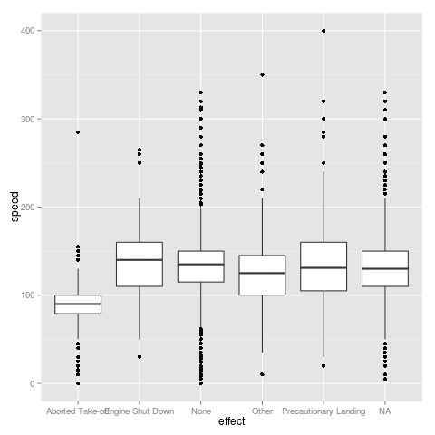
Sometimes when plotting factor variables in R, the graphics can look pretty messy thanks to long factor levels. If the level attributes have multiple words, there is an easy fix to this that often makes the axis labels look much cleaner.

Without Line Breaks

Here's the messy looking example:

No line breaks in axis labels

And here's the code for the messy looking example:

library(OIdata)
data(birds)
library(ggplot2)

ggplot(birds,
  aes(x = effect,
    y = speed)) +
geom_boxplot()

With Line Breaks

We can use regular expressions to add line breaks to the factor levels by substituting any spaces with line breaks:

library(OIdata)
data(birds)
library(ggplot2)

levels(birds$effect) <- gsub(" ", "\n", levels(birds$effect))
ggplot(birds,
  aes(x = effect,
    y = speed)) +
geom_boxplot()

Line breaks in axis labels

Just one line made the plot look much better, and it will carry over to other plots you make as well. For example, you could create a table with the same variable.

Horizontal Boxes

Here we can see the difference in a box plot with horizontal boxes. It's up to you to decide which style looks better:

No line breaks in axis labels

Line breaks in axis labels

library(OIdata)
data(birds)
library(ggplot2)

levels(birds$effect) <- gsub(" ", "\n", levels(birds$effect))
ggplot(birds,
  aes(x = effect,
    y = speed)) +
geom_boxplot() + 
coord_flip()

Just a note: if you're not using ggplot, the multi-line axis labels might overflow into the graph.

The code is available in a gist.

Citations and Further Reading

• http://regex.learncodethehardway.org/

Custom Legend in R

This particular custom legend was designed with three purposes:

• To effectively bin values based on a theoretical minimum and maximum value for that variable (e.g. -1 and 1 or 0 and 100)
• To use a different interval notation than the default
• To handle NA values

Even though this particular legend was designed with those needs, it should be simple to extrapolate from that to build legends based on other criteria.

Standard Legend

For this post, I'll be assuming you've looked through the Oregon map tutorial or have other experience making legends in R. If not, you'll probably want to check that link out. It's an awesome tutorial.

Let's start by creating a map with a standard legend, and then we move on to customization later.

First, we'll load the packages we need and the data from OIdata:

library(OIdata)
library(RColorBrewer)
library(classInt)

# load state data from OIdata package:
data(state)

Next we want to set some constants. This will save us a bunch of typing and will make the code easier to read, especially once we start creating a custom legend. Also, it will allow us to easily change the values if we want a different number of bins or a different min and max.

In this example, we're assuming we have a theoretical minimum and maximum and want to determine our choropleth bins based on that.

nclr <- 8 # number of bins
min <- 0 # theoretical minimum
max <- 100 # theoretical maximum
breaks <- (max - min) / nclr

Next, we'll set up our choropleth colors (this should look familiar from the Oregon tutorial):

# set up colors:
plotclr <- brewer.pal(nclr, "Oranges")
plotvar <- state$coal
class <- classIntervals(plotvar,
  nclr,
  style = "fixed",
  fixedBreaks = seq(min, max, breaks))
colcode <- findColours(class, 
  plotclr)

And now let's map the data:

# map data:
map("state", # base
  col = "gray80",
  fill = TRUE,
  lty = 0)
map("state", # data
  col = colcode,
  fill = TRUE,
  lty = 0,
  add = TRUE)
map("state", # border
  col = "gray",
  lwd = 1.4,
  lty = 1,
  add = TRUE)

And finally let's add our default legend:

legend("bottomleft", # position
  legend = names(attr(colcode, "table")), 
  title = "Percent",
  fill = attr(colcode, "palette"),
  cex = 0.56,
  bty = "n") # border

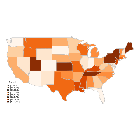
Here's the output of this code (see map-standard-legend.R in the gist):

Percent of power coming from coal sources (standard legend)

Custom Legend

Next we want to add a few lines here and there to enhance the legend.

For starters, let's deal with NA values. We don't have any in this particular dataset, but if we did, we would have seen they were left as the base color of the map and not included in the legend.

After our former code setting up the colors, we should add the color for NAs. It's important that these lines go after all the other set up code, or the wrong colors will be mapped.

# set up colors:
plotclr <- brewer.pal(nclr, "Oranges")
plotvar <- state$coal
class <- classIntervals(plotvar,
  nclr,
  style = "fixed",
  fixedBreaks = seq(min, max, breaks))
colcode <- findColours(class, 
  plotclr)
NAColor <- "gray80"
plotclr <- c(plotclr, NAColor)

We also want to let the map know to have our NA color as the default color, so the map will use that instead of having those areas be transparent:

# map data:
map("state", # base
  col = NAColor,
  fill = TRUE,
  lty = 0)
map("state", # data
  col = colcode,
  fill = TRUE,
  lty = 0,
  add = TRUE)
map("state", # border
  col = "gray",
  lwd = 1.4,
  lty = 1,
  add = TRUE)

Next, we want to set up the legend text. For all but the last interval, we want it to say i ≤ n < (i + breaks). The last interval should be i ≤ n ≤ (i + breaks). This can be accomplished by

# set legend text:
legendText <- c()
for(i in seq(min, max - (max - min) / nclr, (max - min) / nclr)) {
  if (i == max(seq(min, max - (max - min) / nclr, (max - min) / nclr))) {
    legendText <- c(legendText, paste(round(i,3), "\u2264 n \u2264", round(i + (max - min) / nclr,3)))
  } else
    legendText <- c(legendText, paste(round(i,3), "\u2264 n <", round(i + (max - min) / nclr,3))) 
}

But we also want to include NAs in the legend, so we need to add a line:

# set legend text:
legendText <- c()
for(i in seq(min, max - (max - min) / nclr, (max - min) / nclr)) {
  if (i == max(seq(min, max - (max - min) / nclr, (max - min) / nclr))) {
    legendText <- c(legendText, paste(round(i,3), "\u2264 n \u2264", round(i + (max - min) / nclr,3)))
    if (!is.na(NAColor)) legendText <- c(legendText, "NA")
  } else
    legendText <- c(legendText, paste(round(i,3), "\u2264 n <", round(i + (max - min) / nclr,3))) 
}

And finally we need to add the legend to the map:

legend("bottomleft", # position
  legend = legendText, 
  title = "Percent",
  fill = plotclr,
  cex = 0.56,
  bty = "n") # border

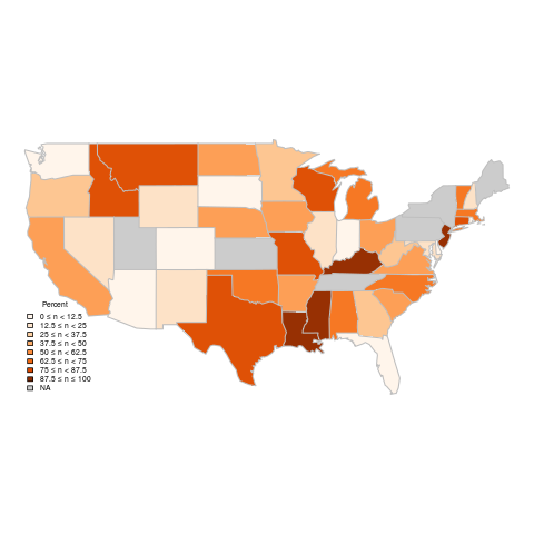
The new map (see map-new-legend.R) meets all the criteria we started with that the original legend didn't have.

Percent of power coming from coal sources (custom legend)

Code is available in a gist.

Citations and Further Reading

• http://geography.uoregon.edu/geogr/topics/maps.htm
• http://stackoverflow.com/questions/13192984/displaying-a-greater-than-or-equal-sign

Perform a Function on Each File in R

Sometimes you might have several data files and want to use R to perform the same function across all of them. Or maybe you have multiple files and want to systematically combine them into one file without having to open each file and manually copy the data out.

Fortunately, it's not complicated to use R to systematically iterate across files.

Finding or Choosing the Names of Data Files

There are multiple ways to find or choose the names of the files you want to analyze.

You can explicitly state the file names or you can get R to find any files with a particular extension.

Explicitly Stating File Names

fileNames <- c("sample1.csv", "sample2.csv")

Finding Files with a Specific Extension

In this case, we use Sys.glob from the base package to find all files including the wildcard "*.csv".

fileNames <- Sys.glob("*.csv")

Iterating Across All Files

We'll start with a loop and then we can add whatever functions we want to the inside of the loop:

for (fileName in fileNames) {

  # read data:
  sample <- read.csv(fileName,
    header = TRUE,
    sep = ",")

  # add more stuff here

}

For example, we could add one to every "Widget" value in each file and overwrite the old data with the new data:

for (fileName in fileNames) {

  # read old data:
  sample <- read.csv(fileName,
    header = TRUE,
    sep = ",")

  # add one to every widget value in every file:
  sample$Widgets <- sample$Widgets + 1
  
  # overwrite old data with new data:
  write.table(sample, 
    fileName,
    append = FALSE,
    quote = FALSE,
    sep = ",",
    row.names = FALSE,
    col.names = TRUE)

}

Or we could do the same thing, but create a new copy of each file:

extension <- "csv"

fileNames <- Sys.glob(paste("*.", extension, sep = ""))

fileNumbers <- seq(fileNames)

for (fileNumber in fileNumbers) {

  newFileName <-  paste("new-", 
    sub(paste("\\.", extension, sep = ""), "", fileNames[fileNumber]), 
    ".", extension, sep = "")

  # read old data:
  sample <- read.csv(fileNames[fileNumber],
    header = TRUE,
    sep = ",")

  # add one to every widget value in every file:
  sample$Widgets <- sample$Widgets + 1
  
  # write old data to new files:
  write.table(sample, 
    newFileName,
    append = FALSE,
    quote = FALSE,
    sep = ",",
    row.names = FALSE,
    col.names = TRUE)

}

In the above example, we used the paste and sub functions from the base package to automatically create new file names based on the old file names.

Or we could instead use each dataset to create an entirely new dataset, where each row is based on data from one file:

fileNames <- Sys.glob("*.csv")

for (fileName in fileNames) {

  # read original data:
  sample <- read.csv(fileName,
    header = TRUE,
    sep = ",")

  # create new data based on contents of original file:
  allWidgets <- data.frame(
    File = fileName,
    Widgets = sum(sample$Widgets))
  
  # write new data to separate file:
  write.table(allWidgets, 
    "Output/sample-allSamples.csv",
    append = TRUE,
    sep = ",",
    row.names = FALSE,
    col.names = FALSE)

}

In the above example, data.frame is used to create a new data row based on each data file. Then the append option of write.table is set to TRUE so that row can be added to the other rows created from other data files.

Those are just a few examples of how you can use R to perform the same function(s) on a large number of files without having to manually run each one. I'm sure you can think of more uses.

All the files are available on GitHub. You can see how eachFile.R, eachfile-newNames.R, and eachFile-append.R each do something different to the sample datasets.

Truncate by Delimiter in R

Sometimes, you only need to analyze part of the data stored as a vector. In this example, there is a list of patents. Each patent has been assigned to one or more patent classes. Let's say that we want to analyze the dataset based on only the first patent class listed for each patent.

patents <- data.frame(
  patent = 1:30,
  class = c("405", "33/209", "549/514", "110", "540", "43", 
  "315/327", "540", "536/514", "523/522", "315", 
  "138/248/285", "24", "365", "73/116/137", "73/200", 
  "252/508", "96/261", "327/318", "426/424/512", 
  "75/423", "430", "416", "536/423/530", "381/181", "4", 
  "340/187", "423/75", "360/392/G9B", "524/106/423"))

We can use regular expressions to truncate each element of the vector just before the first "/".

grep, grepl, sub, gsub, regexpr, gregexpr, and regexec are all functions in the base package that allow you to use regular expressions within each element of a character vector. sub and gsub allow you to replace within each element of the vector. sub replaces the first match within each element, while gsub replaces all matches within each element. In this case, we want to remove everything from the first "/" on, and we want to replace it with nothing. Here's how we can use sub to do that:

patents$primaryClass <- sub("/.*", "", patents$class)

> table(patents$primaryClass)

110 138  24 252 315 327  33 340 360 365 381   4 405 416 423 426  43 430 523 524 
  1   1   1   1   2   1   1   1   1   1   1   1   1   1   1   1   1   1   1   1 
536 540 549  73  75  96 
  2   2   1   2   1   1 

--
This post is one part of my series on Text to Columns.

Citations and Further Reading

• Regular Expressions Cheat Sheet

Only Load Data If Not Already Open in R

I often find it beneficial to check to see whether or not a dataset is already loaded into R at the beginning of a file. This is particularly helpful when I'm dealing with a large file that I don't want to load repeatedly, and when I might be using the same dataset with multiple R scripts or re-running the same script while making changes to the code.

To check to see if an object with that name is already loaded, we can use the exists function from the base package. We can then wrap our read.csv command with an if statement to cause the file to only load if an object with that name is not already loaded.

if(!exists("largeData")) {
  largeData <- read.csv("huge-file.csv",
    header = TRUE)
}

You will probably also find it useful to use the "colClasses" option of read.csv or read.table to help the file load faster and make sure your data are in the right format. For example:

if(!exists("largeData")) {
  largeData <- read.csv("huge-file.csv",
    header = TRUE,
    colClasses = c("factor", "integer", "character", "integer", 
      "integer", "character"))
}

--
This post is one part of my series on dealing with large datasets.

Using colClasses to Load Data More Quickly in R

Specifying a colClasses argument to read.table or read.csv can save time on importing data, while also saving steps to specify classes for each variable later.

For example, loading a 893 MB took 441 seconds to load when not using colClasses, but only 268 seconds to load when using colClasses. The system.time function in base can help you check your own times.

Without specifying colClasses:

   user  system elapsed 
441.224   8.200 454.155 

When specifying colClasses:

   user  system elapsed 
268.036   6.096 284.099 

The classes you can specify are: factor, character, integer, numeric, logical, complex, and Date. Dates that are in the form %Y-%m-%d or Y/%m/%d will import correctly. This tip allows you to import dates properly for dates in other formats.

system.time(largeData <- read.csv("huge-file.csv",
  header = TRUE,
  colClasses = c("character", "character", "complex", 
    "factor", "factor", "character", "integer", 
    "integer", "numeric", "character", "character",
    "Date", "integer", "logical")))

If there aren't any classes that you want to change from their defaults, you can read in the first few rows, determine the classes from that, and then import the rest of the file:

sampleData <- read.csv("huge-file.csv", header = TRUE, nrows = 5)
classes <- sapply(sampleData, class)
largeData <- read.csv("huge-file.csv", header = TRUE, colClasses = classes)
str(largeData)

If you aren't concerned about the time it takes to read the data file, but instead just want the classes to be correct on import, you have the option of only specifying certain classes:

smallData <- read.csv("small-file.csv", 
 header = TRUE,
 colClasses=c("variableName"="character"))

> class(smallData$variableName)
[1] "character"

Citations and Further Reading

• http://stackoverflow.com/questions/2805357/specifying-colclasses-in-the-read-csv
• http://www.biostat.jhsph.edu/~rpeng/docs/R-large-tables.html
• http://www.mollietaylor.com/2013/08/date-formats-in-r.html
• http://stackoverflow.com/a/13022441

--
This post is one part of my series on dealing with large datasets.

Plot Weekly or Monthly Totals in R

When plotting time series data, you might want to bin the values so that each data point corresponds to the sum for a given month or week. This post will show an easy way to use cut and ggplot2's stat_summary to plot month totals in R without needing to reorganize the data into a second data frame.

Let's start with a simple sample data set with a series of dates and quantities:

library(ggplot2)
library(scales)

# load data:
log <- data.frame(Date = c("2013/05/25","2013/05/28","2013/05/31","2013/06/01","2013/06/02","2013/06/05","2013/06/07"), 
  Quantity = c(9,1,15,4,5,17,18))

log

str(log)

> log
        Date Quantity
1 2013/05/25        9
2 2013/05/28        1
3 2013/05/31       15
4 2013/06/01        4
5 2013/06/02        5
6 2013/06/05       17
7 2013/06/07       18

> str(log)
'data.frame': 7 obs. of  2 variables:
 $ Date    : Factor w/ 7 levels "2013/05/25","2013/05/28",..: 1 2 3 4 5 6 7
 $ Quantity: num  9 1 15 4 5 17 18

Next, if the date data is not already in a date format, we'll need to convert it to date format:

# convert date variable from factor to date format:
log$Date <- as.Date(log$Date,
  "%Y/%m/%d") # tabulate all the options here
str(log)

> str(log)
'data.frame': 7 obs. of  2 variables:
 $ Date    : Date, format: "2013-05-25" "2013-05-28" ...
 $ Quantity: num  9 1 15 4 5 17 18

Next we need to create variables stating the week and month of each observation. For week, cut has an option that allows you to break weeks as you'd like, beginning weeks on either Sunday or Monday.

# create variables of the week and month of each observation:
log$Month <- as.Date(cut(log$Date,
  breaks = "month"))
log$Week <- as.Date(cut(log$Date,
  breaks = "week",
  start.on.monday = FALSE)) # changes weekly break point to Sunday
log

> log
        Date Quantity      Month       Week
1 2013-05-25        9 2013-05-01 2013-05-19
2 2013-05-28        1 2013-05-01 2013-05-26
3 2013-05-31       15 2013-05-01 2013-05-26
4 2013-06-01        4 2013-06-01 2013-05-26
5 2013-06-02        5 2013-06-01 2013-06-02
6 2013-06-05       17 2013-06-01 2013-06-02
7 2013-06-07       18 2013-06-01 2013-06-02

Finally, we can create either a line or bar plot of the data by month and by week, using stat_summary to sum up the values associated with each week or month:

# graph by month:
ggplot(data = log,
  aes(Month, Quantity)) +
  stat_summary(fun.y = sum, # adds up all observations for the month
    geom = "bar") + # or "line"
  scale_x_date(
    labels = date_format("%Y-%m"),
    breaks = "1 month") # custom x-axis labels

Time series plot, binned by month

# graph by week:
ggplot(data = log,
  aes(Week, Quantity)) +
  stat_summary(fun.y = sum, # adds up all observations for the week
    geom = "bar") + # or "line"
  scale_x_date(
    labels = date_format("%Y-%m-%d"),
    breaks = "1 week") # custom x-axis labels

Time series plot, totaled by week

The full code is available in a gist.

References

• http://stackoverflow.com/questions/3496536/barplot-totals-by-month-with-ggplot

References

Thursday, February 6, 2014
Thursday, October 24, 2013